Microprice, imbalance, and slippage over batched multi-instrument books.
C · GRAPH RUNTIME · CPU · CUDA · COMPILER · LLVM
Lazy graph based tensor execution runtime
View complete project source on GitHub01 · Architecture
Lazy graph runtime backed by compiled operations
The tensor API builds a lazy computation graph rather than immediately executing each operation. When a value is materialized, the runtime walks the required subgraph, resolves each operation through the JIT cache, and dispatches execution (as a batch) to the selected backend.
Runtime execution
UserTensor API
↓
GraphLazy operation nodes
↓
ExecutionPrepare / dispatch
↓
JIT cacheLookup / compile
↓
BackendCPU · CUDA · generic
Build-time operation compiler
.op definitions
↓
Operation compilerParse · validate · specialize · lower
↓
LLVM bitcode + registry
↓
Tensor library
02 · Graph, memory, JIT
Runtime lifecycle
lifecycle_demo.c
Loading source…


03 · Streamed financial data
Live order books through a persistent tensor graph
A live Binance depth feed maintains 489 order books and presents each retained snapshot as four contiguous tensors. The graph computes imbalance, microprice, and slippage without rebuilding its storage.
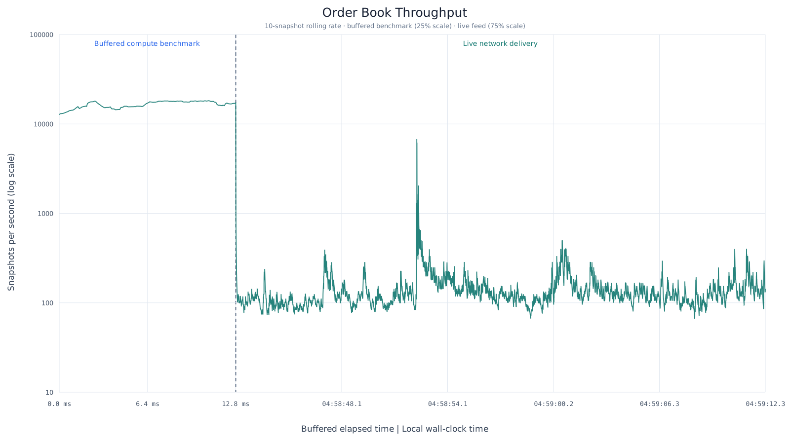
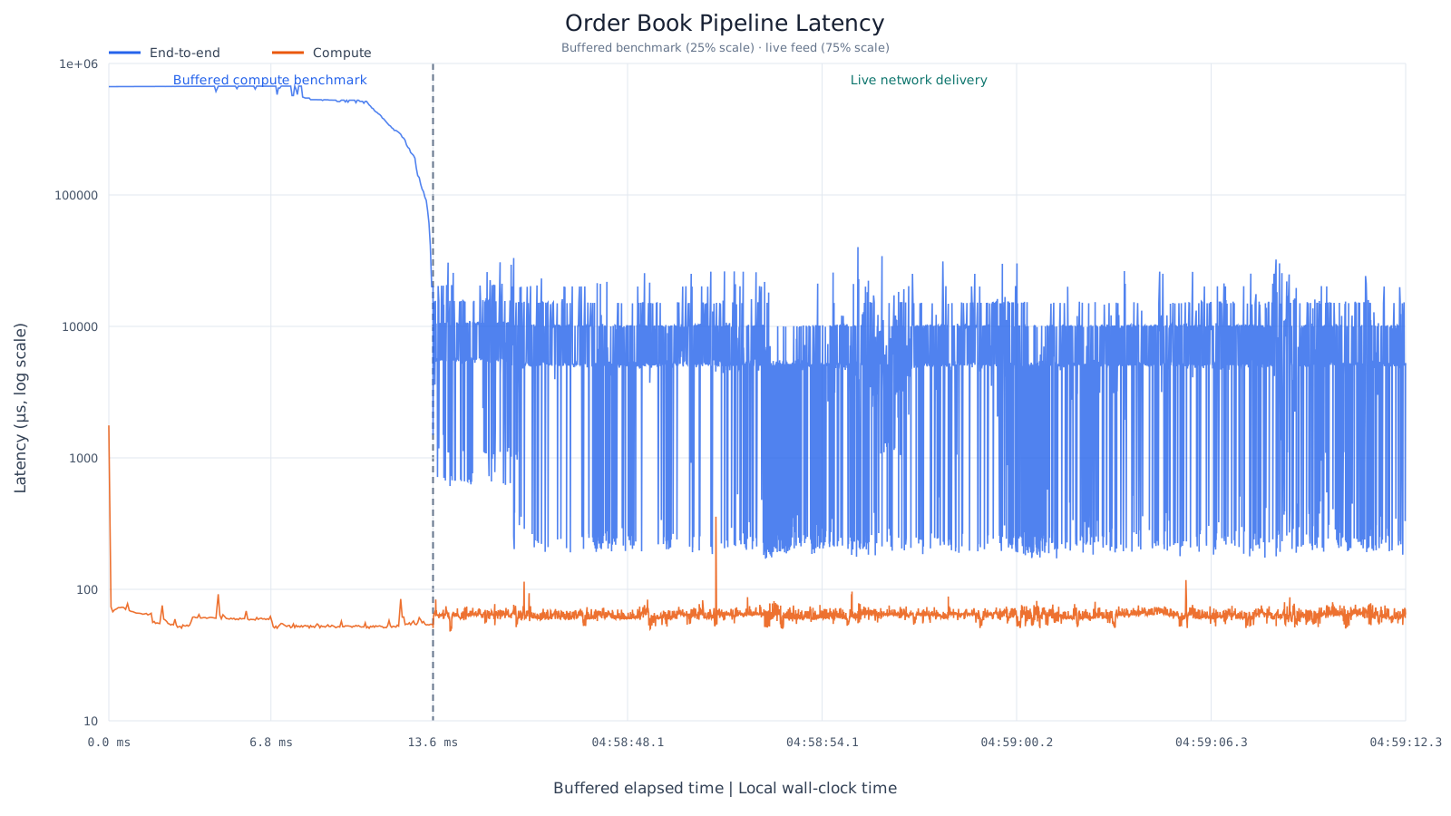
A 224-snapshot retained warm-up separates compute capacity from live arrival rate.
The graph persists; each iteration only rebinds queue-owned input pointers.
A lock-free circular queue hands snapshots to the consumer without a dequeue copy.
Eight WebSocket/parser workers feed one consistent snapshot assembler.
After buffering, throughput is limited by live market arrivals and snapshot assembly.
Finance operation definitions
microprice.op
Loading source…
orderbook_imbalance.op
Loading source…
slippage.op
Loading source…
Streaming application
order_book/main.c
Loading source…
Published implementation
The complete producer, SPSC queue, timing utilities, headers, and application source are available on the artifacts page.
Browse order-book source04 · .op compiler
DSL expands...
You write one generic tensor operation as matrix multiplication, and the compiler generates the concrete C wrappers, LLVM bitcode, and runtime registry for every supported dtype instead of requiring a separate hand written kernel for each one.
matrix_mul.op · source definition
Loading source…
Turns DSL statements and algorithm blocks into compiler input.
Builds an operation AST from types, shapes, algorithms, and hints.
Resolves dimensions, dtypes, IDs, targets, and selection rules.
Expands T = any into concrete dtype kernels.
Materializes pointers, shape bindings, dispatch, and metadata.
Clang lowers generated C into optimizable LLVM IR.
Maps operation IDs and dtype signatures to compiled symbols.
Runtime lookup executes prepared functions without parsing DSL source.
matrix_mul.op defines the operation once using the generic type T = any, symbolic dimensions M, K, and N, and several algorithm implementations. The operation compiler parses and validates the definition, resolves the target for each algorithm, and generates a concrete specialization for each supported dtype.
Each specialization expands into C with the required tensor bindings, concrete pointer types, shape extraction, and algorithm dispatch. Clang then compiles the generated C to LLVM bitcode, while registry.c records how an operation ID and dtype signature map to symbols in that module. The runtime can therefore look up the required implementation directly without parsing the .op source again.
Why it exists: the operation is written once while the compiler generates the repetitive type-specific and runtime integration code around it. The visible trace is an inspection tool that shows the transformation from source through the lexer, AST, validation, generated C, LLVM IR, and registry.
View the complete generated compiler trace
matrix_mul.op → generated C → LLVM bitcode → registry.c
Loading compiler trace…
Why bother?
The purpose of the DSL is not merely to shorten kernel syntax. It moves repetitive implementation work out of every operation and into one compiler.
T = any behaves like a constrained generic type. The
compiler monomorphizes the operation into concrete dtype variants
such as matrix_mul<int32> and
matrix_mul<real32>. Shared symbolic dimensions
become runtime tensor-shape bindings, algorithm metadata becomes
generated dispatch logic, and operation-count expressions become
profiler code.
Without this layer, each operation would need to manually reproduce dtype switches, pointer casts, shape extraction, parameter unpacking, dispatch tables, symbol registration, and profiler metadata.
human-maintained code
        |
        v
compact operation definition
        |
        v
mechanically generated boilerplate
Compiler pipeline
              matrix_mul.op
                    |
                    v
             +-------------+
             |    Lexer    |
             +-------------+
                    |
                    v
        Line / AlgorithmBlock stream
                    |
                    v
             +-------------+
             |   Parser    |
             +-------------+
                    |
                    v
              Operation AST
                    |
                    v
             +-------------+
             |  Validator  |
             +-------------+
                    |
                    v
          ValidatedOperation
                    |
                    v
        +-----------------------+
        | Type specialization   |
        | and C lowering        |
        +-----------------------+
                    |
                    v
              operations.c
                    |
                    v
             clang -emit-llvm
                    |
                    v
              operations.bc
                    |
          +---------+---------+
          |                   |
          v                   v
      LLVM ORC           registry.c
          |                   |
          +---------+---------+
                    |
                    v
             runtime lookup
                    |
                    v
               execution
Frontend · lexical structure
lexer.py performs the first compiler pass. DSL
statements are normalized into logical source lines, while
algorithm bodies are preserved as complete C blocks. A declaration
such as dim M; becomes a lexical line, while an
algorithm block becomes an AlgorithmBlock.
The lexer deliberately does not interpret the C inside an
algorithm; it establishes the outer structure of the operation
language.
Parser · syntax to AST
parser.py converts the lexical stream into an
abstract syntax tree. Definitions such as
type T = any;, dim M;, and
in a: T [M, K]; become structured type definitions,
dimensions, shapes, values, algorithms, and hints under one
Operation node.
Semantic analysis · validation and resolution
validator.py resolves named types and shapes,
verifies dimensions, checks that algorithms and hints agree,
validates operation IDs and names, and resolves backend selection
rules into a ValidatedOperation. This is the compiler
boundary between syntactically valid input and semantically valid
operation metadata. For matrix_mul, it establishes
that all tensors share T and that both occurrences of
K describe the same logical dimension.
Specialization · generic types become concrete kernels
The operation compiler enumerates legal assignments for generic type variables. One source algorithm therefore expands into concrete functions for the supported integer and floating-point types before execution.
matrix_mul<T>
      |
      +--> matrix_mul<int8>
      +--> matrix_mul<int16>
      +--> matrix_mul<int32>
      +--> ...
      +--> matrix_mul<real32>
      +--> matrix_mul<real64>
This is compile-time monomorphization: generic source is expanded into concrete functions before runtime.
Lowering · DSL concepts become C machinery
The lowering pass makes implicit DSL information explicit. For an
int32 specialization, a declaration such as
in a: T [M, K]; becomes a typed input pointer and
concrete shape bindings:
const int32 *restrict a =
    (const int32 *)inputs[0];

extent M = input_tensors[0]->shape[0];
extent K = input_tensors[0]->shape[1];
Output pointers, dimensions, tensor ranks, sizes, parameter
blocks, algorithm conditions, and operation metadata are generated
in the same way. This is why a small .op definition
can expand into a much larger C translation unit: the compiler is
materializing details that would otherwise be handwritten
repeatedly.
LLVM lowering · C becomes SSA-based IR
Clang compiles the generated C into LLVM bitcode. Source variables and loops are represented in LLVM’s SSA-oriented form. The inner matrix accumulation becomes an explicit loop-carried data dependency:
%acc = phi i32 [ 0, %entry ], [ %next_acc, %loop ]
%k   = phi i64 [ 0, %entry ], [ %next_k, %loop ]

%product  = mul i32 ...
%next_acc = add i32 %product, %acc
%next_k   = add i64 %k, 1
The original accumulation,
acc += a[i * K + k] * b[k * N + j], is now explicit
dataflow that LLVM can analyze and optimize.
Registry generation · compiler output becomes runtime-addressable
The generated registry embeds the combined bitcode module and maps
operation identities and dtype signatures to symbols within it.
The runtime does not need to understand .op syntax:
parsing and semantic validation have already happened during the
shared-library build.
Runtime lookup starts from the operation ID, output dtype, and input dtype, then resolves the corresponding function inside the embedded LLVM module.
Build-time language, runtime artifact
LIBRARY BUILD TIME

.op source
   ↓
operation compiler
   ↓
validated / specialized generated code
   ↓
LLVM bitcode + registry
RUNTIME

tensor graph
   ↓
registry lookup
   ↓
LLVM specialization / prepared function
   ↓
execution
The custom language adds compiler structure without requiring the application to parse or interpret DSL source during normal tensor execution.
05 · Execution lifecycle
view_to()
-
When user code is executed,
graph/sketch.crecords the graph using the smallest amount of information needed to reproduce it later, if the work is actually required. -
When the program asks for the actual data,
graph/walker.cwalks the graph from that node and discovers the work required to physically materialize it. Already cached or materialized work is skipped. -
The resulting work queue is sent to the relevant backend: CPU for
packed SIMD and multicore execution, CUDA, or the generic
baseline backend. The backend-specific implementation performs
the execution, while
graph/graph.cwaits for its completion. This materializes only the required subgraph. - Because subgraphs are materialized on demand, dead paths and code are eliminated automatically.
Note:
-
graph/fusion.cprovides safe fusion, including constant folding, transparently rewriting node metadata such as parents, children, and operation IR IDs — but the backend may perform more aggressive fusions. - The walker can prefetch the JIT cache after fusion but before materialization, avoiding duplicate work for fused operations and keeping the cache hot for re-execution.
- If the persistent cache is enabled and hot, the walker reuses it instead of preparing the same kernel again.
06 · IR and JIT cache
Why the cache stores IR, not a function pointer
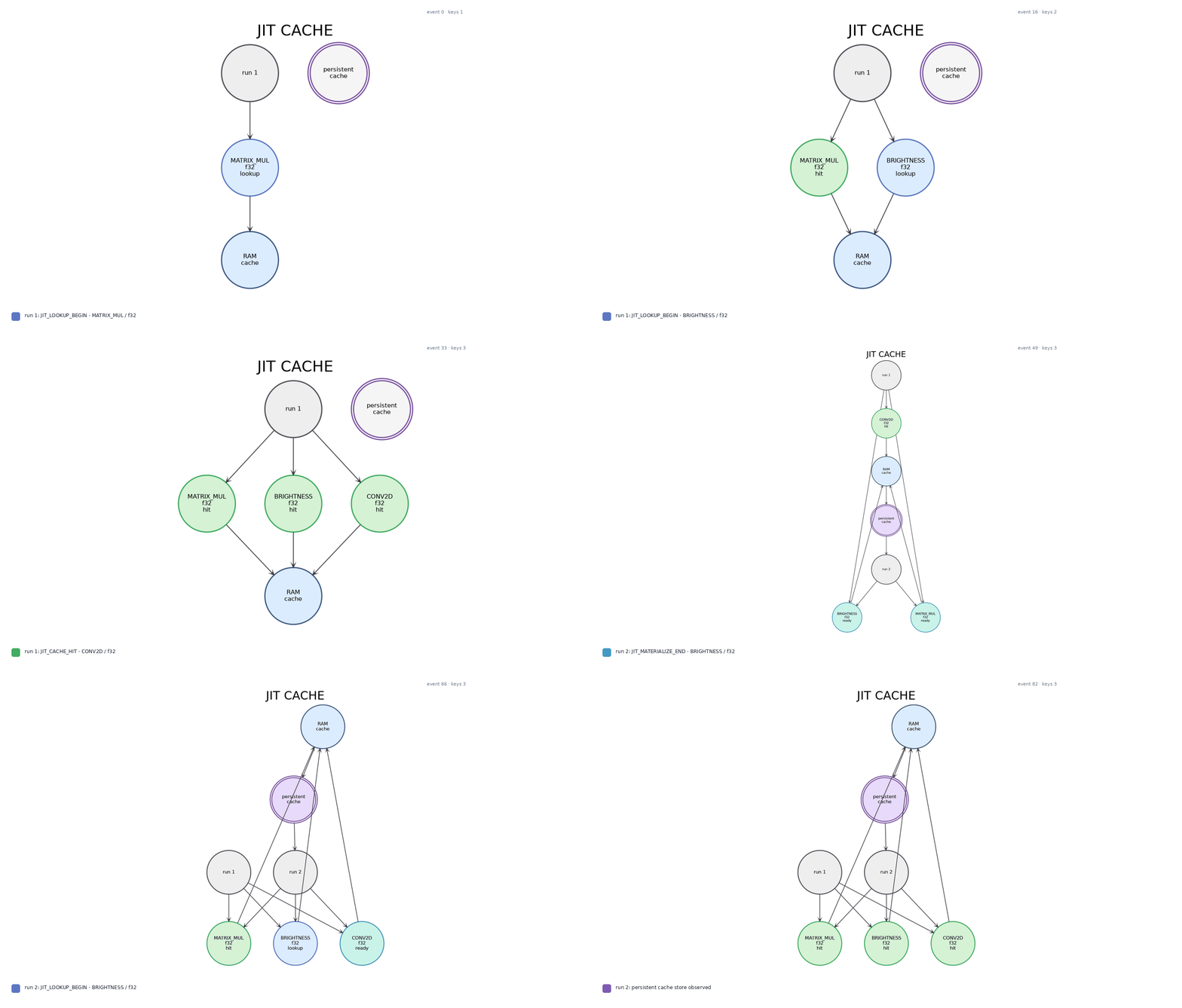
A function pointer is only meaningful inside the process that created it. The persistent cache stores the portable compiled representation and its specialization key instead: operation, dtype, shape, layout, and backend. A later process can load that representation and rebuild a valid executable entry for its own address space.
tests/linalg/main.c · complete source
Loading source…
Why this stresses JIT:
The test requests matrix multiplication and convolution for every
supported dtype, plus matrix inversion for real32 and real64.
Different operation IDs, dtypes, ranks, and shapes produce distinct
JIT-cache keys instead of repeatedly reusing one kernel.
capture · 365.882 msJIT compile work · 361.240 mscache · 24 hits / 22 misses
capture · 4.945 msJIT compile work · 0.000 mscache · 46 hits / 0 misses
View the complete lin_alg profiler reports
Run 1 · CPU · normal JIT cache
Loading report…
Run 2 · CPU · persistent cache
Loading report…
07 · Backends
Backend Implementations
Generic
The correctness baseline. It performs no backend optimization; it executes the submitted work queue for the subgraph one item after another and reports back when the queue is complete.
CPU
The multicore CPU backend uses packed SIMD and LLVM ORC v2 to generate optimized code. Fusion is applied before execution.
A pthread parallelization pass takes scalar SSA and breaks it into worker functions. LLVM’s loop vectorizer and SLP vectorizer then operate on that SSA, after parallelization. The worker pool stays alive across the complete subgraph queue, amortizing operating-system scheduling overhead.
CUDA
This backend also uses LLVM to lower SSA into PTX. It generally creates one kernel for the whole work queue to amortize synchronization and copying between the CPU and CUDA.
Operations are inlined, CUDA parallelization is applied, and grid synchronization separates stages before cooperative launch.
08 · Case study
RAW image signal processing pipeline
The primary demonstration is a complete RAW10 image processing graph. Its stages are implemented as custom domain operations rather than selected from a predefined image processing library.
RAW10 input
BLC
DPC
AWB
Demosaic
CCM
Gamma
Blur
RGB → YUV
NV12

What the application demonstrates
- A substantial graph containing branches, joins, and shared intermediate tensors.
- Domain operations defined outside the runtime through the operation framework.
- Materialization of both RGB preview and NV12 output endpoints.
- JIT specialization for concrete image dimensions, layouts, and data types.
- Lifetime based planning for large image intermediates through the lazy memory pool.
- Combined graph, kernel, memory, JIT, traffic, and operation cost profiling.
View the application source and reconstructed operation graph
main_alt.c · graph construction
Loading source…
Profiler · operation graph
Loading report…
09 · Measured behavior
Runtime behavior confirmed by the integrated profiler
The profiler provides evidence for graph execution, specialization, fusion, and memory behavior.
Graph construction creates nodes without immediately running their kernels. Work begins when a concrete output is requested.
A materialization request walks the dependencies needed for its endpoint rather than executing every node in the graph.
The persistent capture executes each ISP kernel 240 times while retaining the same graph, specialization set, and memory plan. Its JIT cache reaches a 99.5% hit rate after the cold specializations are prepared.
JIT preparation is reported separately from kernel execution, distinguishing initial specialization from later reuse.
Compatible graph nodes appear as a combined kernel entry when the planner legally fuses them.
Reports expose planned bytes, committed storage, logical graph releases, and peak live pool allocation.
Compare single-frame and persistent execution
Single frame · summary and kernel calls
Loading report…
Persistent graph · 240 frames
Loading report…
Single frame · JIT cache
Loading report…
Persistent graph · JIT cache
Loading report…
Note: The presistent cache is diabaled for this demonstration. Both captures prepare the same 11 cold specializations, so total JIT compile work remains nearly constant. The persistent case reuses those functions across 240 materializations: kernel work scales with the frame count, while compile cost and the 538,549,824-byte pool plan are paid once. The loop writes files only for frame 5 because every iteration currently reuses the same RAW input; all 240 frames are still materialized and profiled.
Open the complete primary profiler summary
Loading report…
10 · Earlier application
YOLOv5n inference graph
An earlier version of the runtime executed a complete YOLOv5n forward pass. This version predates the current LLVM JIT and integrated profiler, but it demonstrates that the graph model can support full machine learning inference pipelines as well as image processing workloads.
This demonstration is retained as part of the project's development history. It is not used as evidence for the current JIT, memory planner, or profiler implementation.
11 · Selected artifacts
Source code, operation definitions, traces, and generated outputs
The published artifact set contains the applications, operation definition, profiler captures, test inputs, and generated outputs used in the demonstrations above.
| Artifact | Purpose | Files |
|---|---|---|
| Full ISP pipeline | Primary graph construction, JIT, memory planning, execution, and profiler case study. | source · report · trace |
| Persistent graph loop | Rebinds input storage and materializes both output endpoints for 240 frames while retaining the previously constructed operation graph. | source · report · trace |
| Fusion and view test | Exercises brightness and LUT fusion, slicing, permutation, reshape, channel selection, and dtype conversion. | source · report · trace |
| Operation definition | Typed operation example containing implementation choices, selection constraints, static operation cost, and fusion metadata. | brightness.op |
| Generated outputs | Images produced by the full ISP and image operation graphs. | ISP preview · crop · green channel |